How to create pivot table in Excel 2013

When you process your data in Excel 2013, you can use pivot table feature to analyze your data. So you can review your data easily. Such as, you can analyze sold item in your shop. How to insert pivot table is easy. Check the steps below!

create pivot table

How to create pivot table in Excel 2013
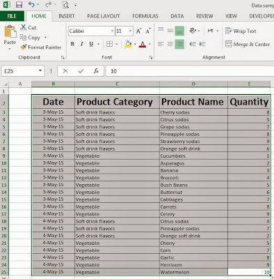
  1. Select all data
  2. insert Pivot table
  3. Click “INSERT”
  4. Click “Pivot Table”
  5. insert Pivot table
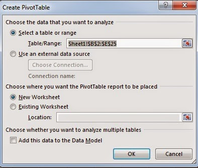
  6. Check that you have select correct tables or ranges and choose where you want to place the pivot table.
  7. insert Pivot table
  8. Click “OK” and the pivot table will place in new worksheet.
  9. Drag the dragging fields to values, rows or column areas.
  10. insert Pivot table
  11. And done.